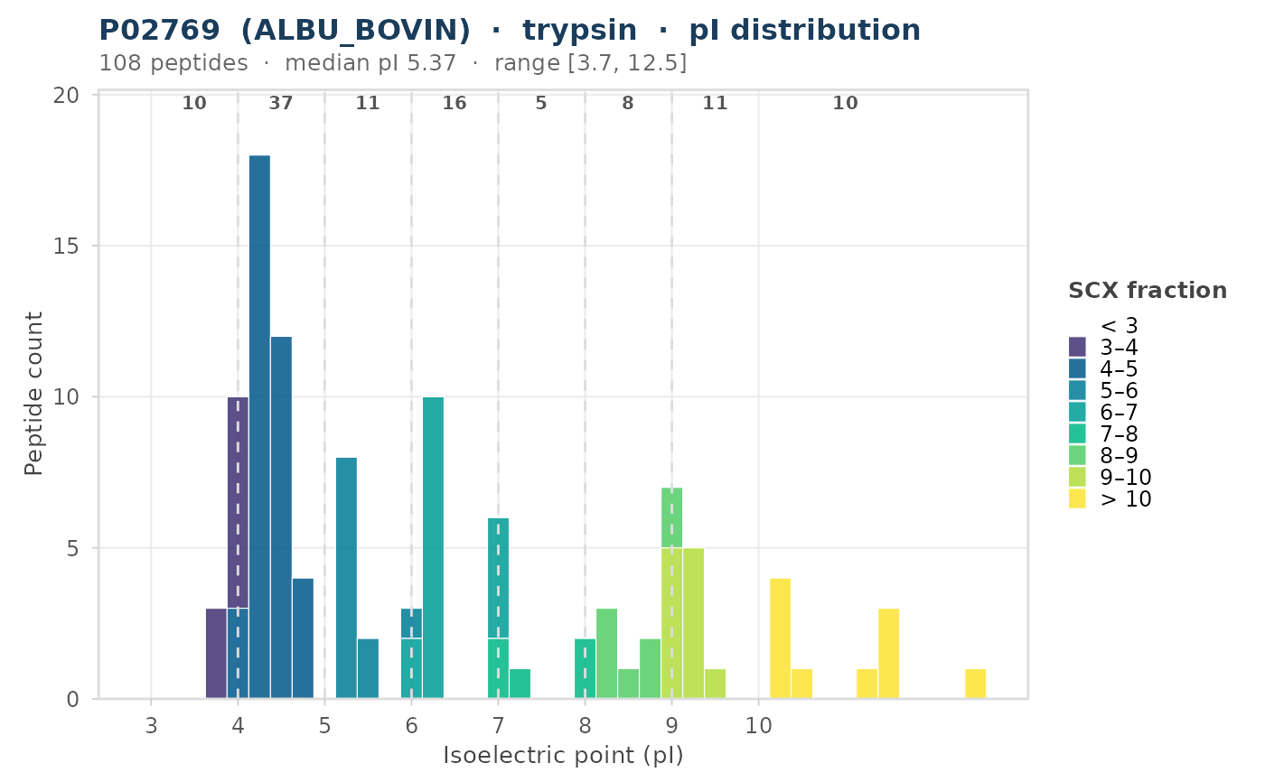
pI Distribution: Histogram of Peptide Isoelectric Points
Source:R/plot_distribution.R
plot_pI_distribution.Rdplot_pI_distribution() draws a histogram of peptide isoelectric points
coloured by SCX fraction bin (e.g., pH 3-4, 4-5, ...) to preview
fractionation outcomes. Vertical boundary lines and per-fraction count
annotations are optionally overlaid.
Usage
plot_pI_distribution(
  result,
  fraction_breaks = c(3, 4, 5, 6, 7, 8, 9, 10),
  show_fraction_lines = TRUE,
  title = NULL
)
Arguments
- result
Accepted inputs:
A named list returned by
evaluate_digest(). pI values are computed automatically from the valid-peptide sequences.A tibble returned by
score_peptides()withinclude_pI = TRUE(contains apIlist column).A plain data.frame / tibble with a numeric
pIcolumn.A bare numeric vector of pI values. If
NULL, raises an error.
- fraction_breaks
Numeric vector of pH boundary values defining the fraction bins. Defaults to
c(3, 4, 5, 6, 7, 8, 9, 10), which produces eight bins:<3,3-4, ...,9-10,>10. IfNULL, raises an error.- show_fraction_lines
Logical. When
TRUE(default) vertical dashed lines are drawn at each interior fraction boundary. IfNULL, treated asFALSE.- title
Optional character string for the plot title. Auto-generated when
NULL(default).
Value
A ggplot object showing a histogram of isoelectric points
coloured by SCX fraction bin with optional fraction boundary lines.
Details
The function accepts four input types with the following
precedence: (1) named list of evaluate_digest() results (multi-input
mode, produces overlaid density curves per result), (2) single
evaluate_digest() result, (3) data.frame with a pI column, (4) raw
numeric vector of pI values. When a full evaluate_digest() result is
supplied, pI values are computed from valid-peptide sequences via
calculate_pI().
See also
evaluate_digest() and score_peptides() for upstream
peptide scoring.
Other plot-distribution:
plot_gravy_landscape(),
plot_length_distribution(),
plot_missed_cleavage_impact(),
plot_mz_distribution()
Examples
if (requireNamespace("ggplot2", quietly = TRUE)) {
  bsa_path <- system.file("extdata", "P02769.fasta", package = "pepVet")
  res <- evaluate_digest(bsa_path, enzyme = "trypsin")
  p <- plot_pI_distribution(res)
  print(p)
}