Score Diagnostics for pepVet Scoring Models

pepVet’s scoring model combines five or six component scores into a weighted composite. The components describe different digest properties, but the formula does not require them to be statistically independent. score_diagnostics() reports multicollinearity, principal components, and the score change produced by setting one component to zero.

Run the diagnostics

The workflow first creates a batch result and then passes that table to score_diagnostics().

Setup

Evaluate the 50-protein fixture with trypsin. This gives a batch result with five component scores per protein.

batch <- batch_evaluate(small_fasta, enzyme = "trypsin")
dim(batch)
#> [1] 50 16

Running diagnostics

A single call to score_diagnostics() runs all three analyses:

d <- score_diagnostics(batch)

The result is a list with six elements. The three analysis results are in $vif, $pca, and $ablation.

names(d)
#> [1] "vif"          "pca"          "ablation"     "n_proteins"   "n_components"
#> [6] "weights"

Diagnostic outputs

The returned object contains three numerical analyses and a plot that presents them together.

VIF: multicollinearity

Variance Inflation Factor measures how much linear dependence on the other components inflates the variance associated with each component score. For each component, the function fits a linear model from the remaining components and computes VIF = 1 / (1 - R^2).

The plot uses VIF values of 5 and 10 as visual reference lines. They are rules of thumb, not pass or fail boundaries. O’Brien (2007) cautions against treating fixed VIF cutoffs as automatic evidence that a model requires correction.

d$vif
#>   S_length S_coverage    S_count    S_hydro   S_charge 
#>   5.776149   2.972499   4.640217   1.688987   2.203141

Components with VIF above 5 receive a plot flag. In this fixture, S_length has VIF = 5.78. This value should prompt inspection of the component relationships and intended model use, not automatic removal of a component.

PCA: dimensionality

Principal component analysis expresses variation in the component matrix through linear combinations. The plot includes an 80% cumulative-variance reference line for description. It is not a model-validity threshold.

round(d$pca$var_explained, 3)
#> [1] 0.675 0.157 0.099 0.049 0.021

In this fixture, PC1 + PC2 explain 83% of variance. The scree plot shows how quickly the remaining variance declines. PCA alone does not establish that each component contributes unique experimental information.

The loadings matrix shows which original components contribute to each PC. PC1 is a weighted average of all five components (all loadings positive, ranging from 0.34 to 0.50). In this sample, PC2 is driven primarily by hydrophobicity (loading -0.86), which is less aligned with the other component loadings on that axis.

PCA loadings (rotation matrix)

	PC1	PC2	PC3	PC4	PC5
S_length	0.500	0.066	0.437	0.008	0.744
S_coverage	0.448	0.499	-0.132	-0.682	-0.260
S_count	0.493	0.076	0.388	0.523	-0.572
S_hydro	0.339	-0.861	-0.003	-0.351	-0.146
S_charge	0.438	-0.006	-0.800	0.372	0.172

Ablation: weighted score contribution

Ablation sets each component to zero without renormalizing the other weights. It reports the resulting composite-score drop and verdict changes. Because the composite is a weighted sum, this analysis describes influence under the current weights rather than empirical importance.

d$ablation
#>    component weight  mean_drop    sd_drop   max_drop n_verdict_flipped
#> 1   S_length  0.200 0.09700884 0.01976096 0.12432432                26
#> 2 S_coverage  0.348 0.23973064 0.06094034 0.34124272                45
#> 3    S_count  0.226 0.20766686 0.04160020 0.22600000                43
#> 4    S_hydro  0.138 0.08726940 0.01952765 0.12075000                20
#> 5   S_charge  0.088 0.06177470 0.01058011 0.07372973                14

Key patterns to look for:

• Mean drop: the score is a weighted sum, so the drop equals the active weight multiplied by the observed component value. In this sample, S_coverage produces the largest mean drop at 0.240, while S_charge produces the smallest at 0.062. This describes the current weights and data. It does not show that the weights are empirically fitted.

• SD drop: the standard deviation reports how much the score drop varies across proteins. In this fixture, the value is largest for S_coverage at 0.061.

• Verdict flips: the count reports how many proteins change label in the zero-component calculation. S_coverage changes 45 of 50 labels, while S_charge changes 14. These counts depend on the current weights, thresholds, and fixture.

The diagnostics plot

plot_score_diagnostics() produces a three-panel figure combining all three analyses:

if (requireNamespace("ggplot2", quietly = TRUE) &&
    requireNamespace("patchwork", quietly = TRUE)) {
  p <- plot_score_diagnostics(d)
  print(p)
}

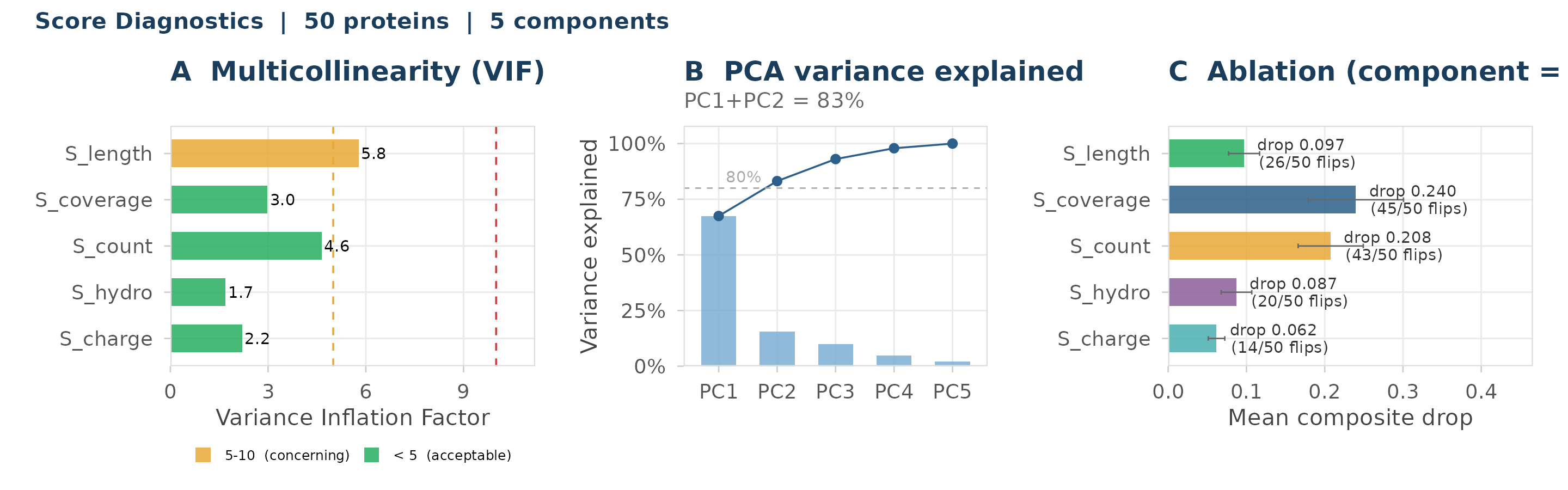
Panel A (VIF): Bars show VIF values. Dashed lines at 5 and 10 mark the package’s reference bands. Values above a band warrant inspection in context.

Panel B (PCA): Bar heights show the variance explained by each principal component. The cumulative line shows total variance explained through each component. The dashed 80% line is a descriptive reference.

Panel C (Ablation): Bars show the mean composite drop when the calculation sets each component to zero. Error bars show plus or minus one standard deviation. The annotation gives the drop and number of verdict changes. This panel does not determine whether to remove or reweight a component.

Interpreting the results

Reference patterns

• VIF values relative to the displayed 5 and 10 reference bands.
• Cumulative variance relative to the displayed 80% reference line.
• Ablation drops relative to the current weights and observed component values.
• Verdict changes relative to the current 0.40 and 0.65 boundaries.

What to do if VIF is high

A high VIF shows that the component is linearly predictable from the other components in the supplied data. Inspect the component definitions, pairwise correlations, sample composition, and intended use before changing the score. Expert-prior weighting does not remove multicollinearity.

When to run diagnostics

Run score_diagnostics() whenever you:

• Change the default weights or add a new component.
• Want to describe score-component relationships in a new proteome.
• Need to document component relationships in a specified dataset.
• Suspect that two components may be measuring the same thing (for example, if S_count and S_coverage behave similarly on a particular enzyme).

References

O’Brien RM. A Caution Regarding Rules of Thumb for Variance Inflation Factors. Quality & Quantity. 2007;41(5):673-690. doi: 10.1007/s11135-006-9018-6.

Session info

sessionInfo()
#> R version 4.6.1 (2026-06-24)
#> Platform: x86_64-pc-linux-gnu
#> Running under: Ubuntu 24.04.4 LTS
#> 
#> Matrix products: default
#> BLAS:   /usr/lib/x86_64-linux-gnu/openblas-pthread/libblas.so.3 
#> LAPACK: /usr/lib/x86_64-linux-gnu/openblas-pthread/libopenblasp-r0.3.26.so;  LAPACK version 3.12.0
#> 
#> locale:
#>  [1] LC_CTYPE=C.UTF-8       LC_NUMERIC=C           LC_TIME=C.UTF-8       
#>  [4] LC_COLLATE=C.UTF-8     LC_MONETARY=C.UTF-8    LC_MESSAGES=C.UTF-8   
#>  [7] LC_PAPER=C.UTF-8       LC_NAME=C              LC_ADDRESS=C          
#> [10] LC_TELEPHONE=C         LC_MEASUREMENT=C.UTF-8 LC_IDENTIFICATION=C   
#> 
#> time zone: UTC
#> tzcode source: system (glibc)
#> 
#> attached base packages:
#> [1] stats     graphics  grDevices utils     datasets  methods   base     
#> 
#> other attached packages:
#> [1] pepVet_0.99.0
#> 
#> loaded via a namespace (and not attached):
#>  [1] gtable_0.3.6         jsonlite_2.0.0       compiler_4.6.1      
#>  [4] crayon_1.5.3         Biostrings_2.81.5    jquerylib_0.1.4     
#>  [7] scales_1.4.0         systemfonts_1.3.2    IRanges_2.47.2      
#> [10] Seqinfo_1.3.0        textshaping_1.0.5    yaml_2.3.12         
#> [13] fastmap_1.2.0        ggplot2_4.0.3        R6_2.6.1            
#> [16] XVector_0.53.0       cleaver_1.51.0       labeling_0.4.3      
#> [19] patchwork_1.3.2      generics_0.1.4       knitr_1.51          
#> [22] BiocGenerics_0.59.10 tibble_3.3.1         desc_1.4.3          
#> [25] RColorBrewer_1.1-3   bslib_0.11.0         pillar_1.11.1       
#> [28] rlang_1.3.0          cachem_1.1.0         xfun_0.60           
#> [31] S7_0.2.2             fs_2.1.0             sass_0.4.10         
#> [34] otel_0.2.0           cli_3.6.6            withr_3.0.3         
#> [37] pkgdown_2.2.1        magrittr_2.0.5       digest_0.6.39       
#> [40] grid_4.6.1           lifecycle_1.0.5      S4Vectors_0.51.5    
#> [43] vctrs_0.7.3          evaluate_1.0.5       glue_1.8.1          
#> [46] farver_2.1.2         ragg_1.5.2           stats4_4.6.1        
#> [49] rmarkdown_2.31       tools_4.6.1          pkgconfig_2.0.3     
#> [52] htmltools_0.5.9